
Plotting NumPy arrays directly using Matplotlib was simple, but what I really wanted though was to show the data in a projected coordinate system. With a little bit of searching it seemed like the Python basemap module should be able to handle this task pretty easily. The examples on the basemap website were really good but the example on Peak5398’s Introduction to Python site also really helped with some of the details.
Just like last time, the first step was reading in the PRISM ASCII raster to a NumPy array. The only difference is that I read the data into a masked array.
import numpy as np

# Read in PRISM header data
prism_name = 'us_tmax_2011.14.asc'
with open(prism_name, 'r') as prism_f:
    prism_header = prism_f.readlines()[:6]

# Pull out nodata value from ASCII raster header
prism_header = [item.strip().split()[-1] for item in prism_header]
prism_cols = int(prism_header[0])
prism_rows = int(prism_header[1])
prism_xll = float(prism_header[2])
prism_yll = float(prism_header[3])
prism_cs = float(prism_header[4])
prism_nodata = float(prism_header[5])

# Readin the PRISM array
prism_array = np.loadtxt(prism_name, dtype=np.float, skiprows=6)

# Build a masked array
prism_ma = np.ma.masked_equal(prism_array, prism_nodata)

# PRISM data is stored as an integer but scaled by 100
prism_ma *= 0.01

# Calculate the extent of the PRISM array
# XMin, XMax, YMin, YMax
prism_extent = [
    prism_xll, prism_xll + prism_cols * prism_cs,
    prism_yll, prism_yll + prism_rows * prism_cs]
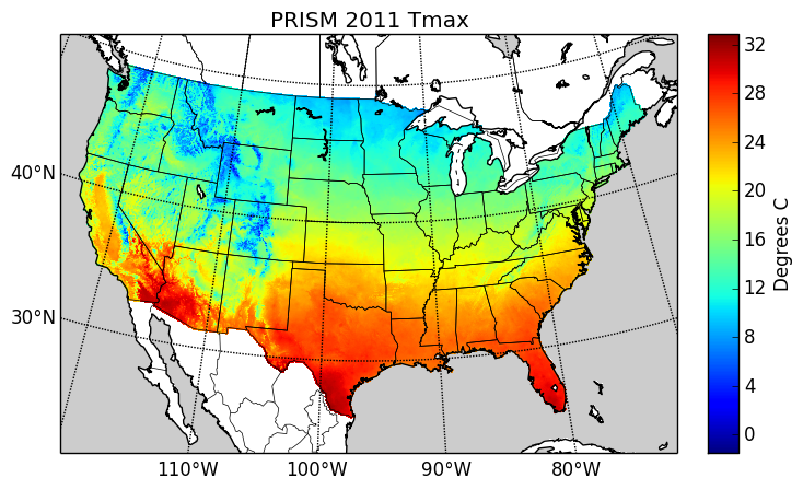
I choose to use an Albers Equal Area projection, but it seems really simple to set just about any projection. I used a masked array so that I could use the maskoceans function to remove the PRISM values over the ocean. Just setting these cells to NaN didn’t work.
Overall it seems really easy to plot array data in a projected coordinate system.
import matplotlib.pyplot as plt
from mpl_toolkits.basemap import Basemap, maskoceans

# Build arrays of the lat/lon points for each cell
lons = np.arange(prism_extent[0], prism_extent[1], prism_cs)
lats = np.arange(prism_extent[3], prism_extent[2], -prism_cs)
lons, lats = np.meshgrid(lons, lats)

# Just the contingous United States
m = Basemap(
    width=5000000, height=3400000, projection='aea', resolution='l',
    lat_1=29.5, lat_2=45.5, lat_0=38.5, lon_0=-96.)

# Build the figure and ax objects
fig, ax = plt.subplots()
ax.set_title('PRISM 2011 Tmax')

# Built-in map boundaries
m.drawcoastlines()
m.drawlsmask(land_color='white', ocean_color='0.8', lakes=False)
m.drawcountries()
m.drawstates()

# Set ocean pixels to nodata
prism_ma_land = maskoceans(lons, lats, prism_ma)

# Draw PRISM array directly to map
im = m.pcolormesh(lons, lats, prism_ma_land, cmap=plt.cm.jet, latlon=True)

# Build the colorbar on the right
cbar = m.colorbar(im, 'right', size='5%', pad='5%')
# Build the colorbar on the bottom
# cbar = m.colorbar(im, 'bottom', size='5%', pad='8%')
cbar.set_label('Degrees C')

# Meridians & Parallels
m.drawmeridians(np.arange(0, 360, 10), labels=[False,False,False,True])
m.drawparallels(np.arange(-90, 90, 10), labels=[True,False,False,False])

# Save and show
plt.show()
